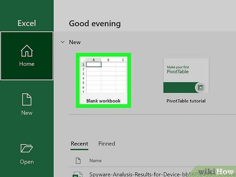
Create or open a workbook. When people refer to “Excel files,” they are referring to workbooks, which are files that contain one or more sheets of data on individual tabs. Each tab is called a worksheet or spreadsheet, both of which are used interchangeably. When you open Excel, you’ll be prompted to open or create a workbook.
To start from scratch, click Blank workbook. Otherwise, you can open an existing workbook or create a new one from one of Excel’s helpful templates, such as those designed for budgeting.
Explore the worksheet. When you create a new blank workbook, you’ll have a single worksheet called Sheet1 (you’ll see that on the tab at the bottom) that contains a grid for your data. Worksheets are made of individual cells that are organized into columns and rows.
Columns are vertical and labeled with letters, which appear above each column.
Rows are horizontal and are labeled by numbers, which you’ll see running along the left side of the worksheet.
Every cell has an address which contains its column letter and row number. For example, the top-left cell in your worksheet’s address is A1 because it’s in column A, row 1.
A workbook can have multiple worksheets, all containing different sets of data. Each worksheet in your workbook has a name—you can rename a worksheet by right-clicking its tab and selecting Rename.
To add another worksheet, just click the + next to the worksheet tab(s).
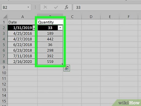
Click a cell to select it. When you click a cell, it will highlight to indicate that it’s selected.
When you type something into a cell, the input text is called a value. Entering data into Excel is as simple as typing values into each cell.
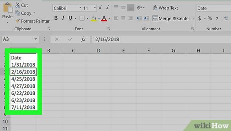
When entering data, the first row of your worksheet (e.g., A1, B1, C1) is typically used as headers for each column. This is helpful when creating graphs or tables which require labels.
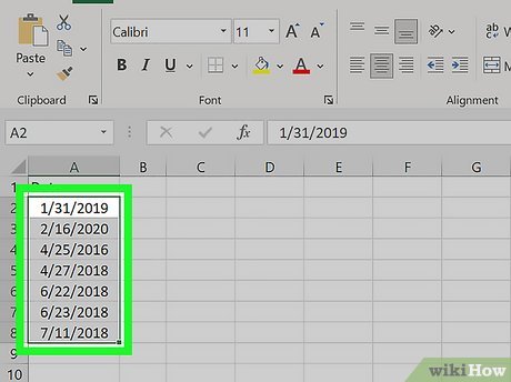
For example, if you’re adding a list of dates in column A, you might click cell A1 and type Date into the cell as the column header.
Type a word or number into the cell. As you’re typing, you’ll see the letters and/or numbers appear in the cell, as well as in the formula bar at the top of the worksheet.
When you start practicing more advanced Excel features like creating formulas, this bar will come in handy.
You can also copy and paste text from other applications into your worksheet, tables from PDFs and the web.
Automatically fill columns based on existing data. Let’s say you want to make a list of consecutive dates or numbers. Or what if you want to fill a column with many of the same values that follow a pattern? As long as Excel can recognize some sort of pattern in your data, such as a particular order, you can use Autofill to automatically populate data into the rest of your column. Here’s a trick to see it in action.
In a blank column, type 1 into the first cell, 2 into the second cell, and then 3 into the third cell.
Hover your mouse cursor over the bottom-right corner of the last cell in your series—it will turn to a crosshair.
Click and drag the crosshair down the column, then release the mouse button once you’ve gone down as far as you like. By default, this will fill the remaining cells with the value of the selected cell—at this point, you’ll probably have something like 1, 2, 3, 3, 3, 3, 3, 3.
Click the small icon at the bottom-right corner of the filled data to open AutoFill options, and select Fill Series to automatically detect the series or pattern. Now you’ll have a list of consecutive numbers. Try this cool feature out with different patterns!
Once you get the hang of AutoFill, you’ll have to try flash fill, which you can use to join two columns of data into a single merged column.
Adjust the column sizes so you can see all of the values. Sometimes typing long values into a cell hides the value and displays hash symbols ### instead of what you’ve typed. If you want to be able to see everything, you can snap the cell contents to the width of the widest cell. For example, let’s say we have some long values in column B:
To expand the contents of column B, hover the cursor over the dividing line between the B and C at the top of the worksheet—once your cursor is right on the line, it will turn to two arrows pointing in either direction.[2] X
Trustworthy Source
Microsoft Support Technical support and product information from Microsoft.
Click and drag the separator until the column is wide enough to accommodate your data, or just double-click the separator to instantly snap the column to the size of the widest value.
Wrap text in a cell. If your longer values are now awkwardly long, you can enable text wrapping in one or more cells. Just click a cell (or drag the mouse to select multiple cells), click the Home tab, and then click Wrap Text on the toolbar.
Edit a cell value. If you need to make a change to a cell, you can double-click the cell to activate the cursor, and then make any changes you need. When you’re finished, just press Enter or Return again.
To delete the contents of a cell, click the cell once and press delete on your keyboard.
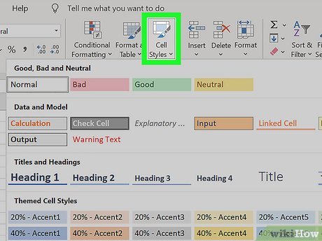
Apply styles to your data. Whether you want to highlight certain values with color so they stand out or just want to make your data look pretty, changing the colors of cells and their containing values is easy—especially if you’re used to Microsoft Word:
Select a cell, column, row, or multiple cells at once.
On the Home tab, click Cell Styles if you’d like to quickly apply quick color styles.
If you’d rather use more custom options, right-click the selected cell(s) and select Format Cells. Then, use the colors on the Fill tab to customize the cell’s background, or the colors on the Font tab for value colors.
Apply number formatting to cells containing numbers. If you have data that contains numbers such as prices, measurements, dates, or times, you can apply number formatting to the data so it will display consistently.[3] X
Trustworthy Source
Microsoft Support Technical support and product information from Microsoft.
By default, the number format is General, which means numbers display exactly as you type them.
Select the cell you want to format. If you’re working with an entire column or row, you can just click the column letter or row number to select the whole thing.
On the Home tab, click the drop-down menu at the top-center—it’ll say General by default, unless you selected cells that Excel recognizes as a different type of number like Currency or Time.
Choose one of the formatting options in the list, such as Short Date or Percentage, or click More Number Formats at the bottom to expand all options (we recommend this!).
If you selected More Number Formats, the Format Cells dialog will expand to the Number tab, where you’ll see several categories for number types.
Select a category, such as Currency if working with money, or Date if working with dates. Then, choose your preferences, such as a currency symbol and/or decimal places.
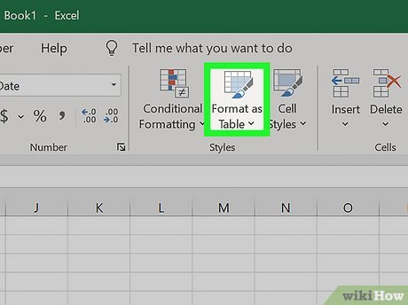
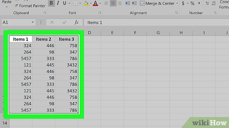
Start by highlighting the values you’ve entered so far, including your column headers. Tables also make it easy to sort and filter your data based on values.
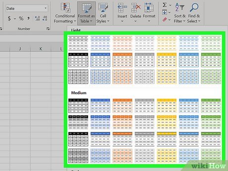
Tables traditionally apply different or alternating colors to every other row for easy viewing. Many table options also add borders between cells and/or columns and rows.
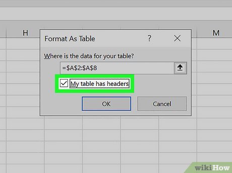
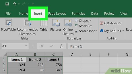
Make sure “My table has headers” is selected and click OK. This tells Excel to turn your column headers into drop-down menus that you can easily sort and filter. Once you click OK, you’ll see that your data now has a color scheme and drop-down menus.
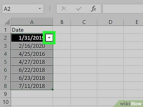
Click the drop-down menu at the top of a column. Now you’ll see options for sorting that column, as well as several options for filtering all of your data based on its values.
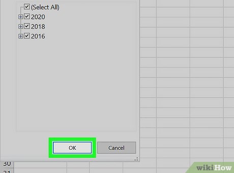
Choose which data to display based on values in this column. The simplest way to do this is to uncheck the values you don’t want to display—if you uncheck a particular date, for example, you’ll prevent rows that contain the selected date in from appearing in your data. You can also use Text Filters or Number Filters, depending on the type of data in the column:
If you chose a numerical column, select Number Filters, then choose an option like Greater Than… or Does Not Equal to be extra specific about which values to hide.
For text columns, you can choose Text Filters, where you can specify things like Begins with or Contains.
Click OK. Your data is now filtered based on your selections. You’ll also see a small funnel icon in the drop-down menu, which indicates that the data is filtering out certain values.
To unfilter your data, click the funnel icon, click Clear filter from (column name), and then click OK.
You can also filter columns that aren’t in tables. Just select a column and click Filter on the Data tab to add a drop-down to that column.
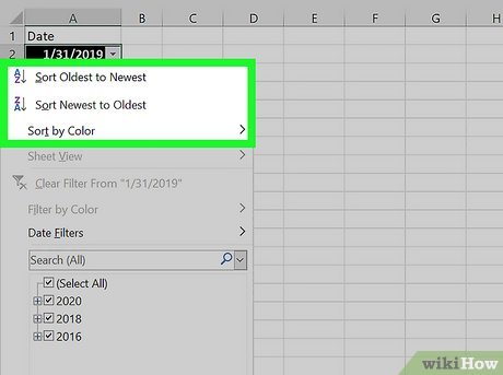
Sort your data in ascending or descending order. Click the drop-down arrow at the top of a column to view sorting options—these allow you to sort all of your data in order based on the current column.
If you’re working with numbers, click Smallest to Largest to sort in ascending order, or Largest to Smallest for descending order.[6] X
Trustworthy Source
Microsoft Support Technical support and product information from Microsoft.
If you’re working with text values, Sort A to Z will sort in ascending order, while Sort Z to A will sort in reverse.
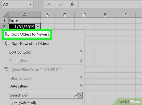
When it comes to sorting dates and times, Sort Oldest to Newest will sort with the earliest date at the top and the oldest date at the bottom, and Newest to Oldest displays the dates in descending order.
When you sort a column, all other columns in the table adjust based on the sort.
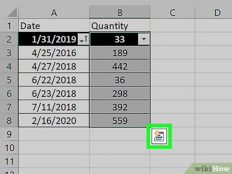
Select the data in your worksheet. Excel’s Quick Analysis feature is the easiest way to perform basic calculations (including totals, averages, and counts) and create meaningful tables or graphs without the need for advanced Excel knowledge.[7] X
Trustworthy Source
Microsoft Support Technical support and product information from Microsoft.
Click the Quick Analysis icon. This is the small icon that pops up at the bottom-right corner of your selection. It looks like a window with some colored lines.
Select an analysis type. You’ll see several tabs running along the top of the window, each of which gives you different option for visualizing your data:
For math calculations, click the Totals tab, where you can select Sum, Average, Count, %Total, or Running Total. You’ll be able to choose whether to display the results at the bottom of each column or to the right.
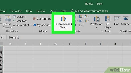
To create a chart, click the Charts tab, then select a chart to visualize your data. Before you settle on a chart, just hover the cursor over each option to see a preview.
To add quick chart data to individual cells, click the Sparklines tab and choose a format. Again, you can hover the cursor over each option to see a preview.
To instantly apply conditional formatting (which is usually a little more complex in Excel) based on your data, use the Formatting tab. Here you can choose an option like Color or Data Bars, which apply colors to your data based on trends.
Quickly add data with AutoSum. AutoSum is a built-in Excel function that makes it easy to find the total of one or more columns in a few clicks. Functions or formulas that perform calculations and other tasks based on the values of cells. When you use a function to get something done, you’re creating a formula, which is like a math equation. If you have a column or row of numbers you want to add:
Click the cell below the numbers you want to add (if a column) or to the right (if a row).[8] X
Trustworthy Source
Microsoft Support Technical support and product information from Microsoft.
On the Home tab, click AutoSum toward the upper-right corner of the app. A formula beginning with =SUM(cell+cell) will appear in the field, and a dotted line will surround the numbers you’re adding.
Press Enter or Return. You should now see the total of the numbers in the selected field. This is here because you created your first formula—which you didn’t have to write by hand!
If you change any numbers in your data after using AutoSum, the AutoSum value will update automatically.
Write a simple math formula. AutoSum is just the beginning—Excel is famous for its ability to do all sorts of simple and complex math calculations on data. Fortunately, you don’t have to be a math whiz to create simple formulas to create everyday math formulas, like adding, subtracting, and multiplying. Here’s some basic formulas to get you started:
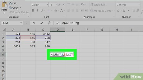
Add: — Type =SUM(cell+cell) (e.g., =SUM(A3+B3)) to add two cells’ values together, or type =SUM(cell,cell,cell) (e.g., =SUM(A2,B2,C2)) to add a series of cell values together.
If you want to add all of the numbers in a whole column (or in a section of a column), type =SUM(cell:cell) (e.g., =SUM(A1:A12)) into the cell you want to use to display the result.
Subtract: Type =SUM(cell-cell) (e.g., =SUM(A3-B3)) to subtract one cell value from another cell’s value.
Divide: Type =SUM(cell/cell) (e.g., =SUM(A6/C5)) to divide one cell’s value by another cell’s value.
Multiply: Type =SUM(cell*cell) (e.g., =SUM(A2*A7)) to multiply two cell values together.
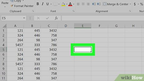
Select a cell for an advanced formula. What if you need to do something more complicated than just adding numbers? Even if you don’t know how to write formulas by hand, you can still create useful formulas that work with your data in various ways. Start by clicking the cell in which you want to display your formula.
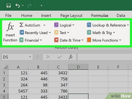
Explore the Function Library. Several function categories appear in the toolbar, such as Financial, Text, and Math & Trig. Click the options to check out the types of functions available, though they might not make a whole lot of sense just yet.
Click Insert Function. This option is in the far-left side of the Formulas toolbar. This opens the Insert Function window, which gives you a more detailed breakdown of each function.
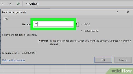
Click a function to learn about it. You can type what you want to do (such as round), or choose a category to filter the list of functions. Then, click any function to read a description of how it works and view its syntax.
For example, to select the formula for finding the tangent of an angle, you would scroll down and click the TAN option.
Fill out the function’s formula. When prompted, type in the number or select a cell for which you want to use the formula.
For example, if you select the TAN function, you’ll type in the number for which you want to find the tangent, or select the cell that contains that number.
Depending on your selected function, you may need to click through a couple of on-screen prompts.
Set up the chart’s data. If you’re creating a line graph or a bar graph, for example, you’ll want to use one column of cells for the horizontal axis and one column of cells for the vertical axis. The best way to do this is to place your data in a table.
Typically speaking, the left column is used for the horizontal axis and the column immediately to the right of it represents the vertical axis.
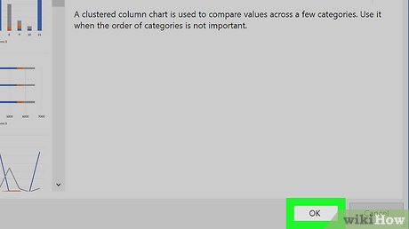
Select a chart template. Click the chart template you want to use based on the type of data you’re working with. If you don’t see a chart type you like, click the All Charts tab to explore by category, such as Pie, Bar, and X Y Scatter.
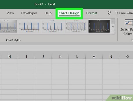
Use the Chart Design tab to customize your chart. Any time you click your chart, the Chart Design tab will appear at the top of Excel. You can adjust the chart style here, change colors, and add additional elements.
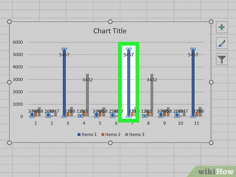
Double-click a chart element to manage it in the Format panel. When you double-click something on your chart, such as a value, line, or bar, you’ll see options you can edit in the panel on the right side of excel. Here you can change the axis labels, alignment, and legend data.
Video
By using this service, some information may be shared with YouTube.
Tips
Submit a Tip
All tip submissions are carefully reviewed before being published


